Our Notebooks integration started as an experimental project, but quickly became a central piece of our Portal experience.

Looking at its exponential growth and our product roadmap (jobs, dashboard apps, etc.) we knew we had to make its experience perfect. Unfortunately, it was more common than we would like to get complaints like, “why is my Notebooks UI taking more than 30 seconds to load?” — especially by people located far away from our control plane infrastructure.
Spoiler: We managed to make our Notebooks UI open in less than a second for some cases. Keep reading to learn more about all the optimizations we have been doing!
How our Notebooks work
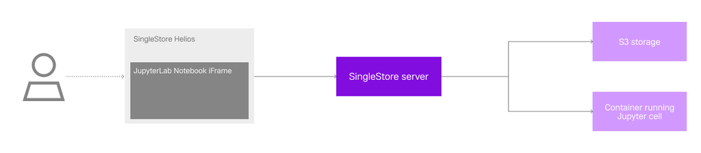
Before diving into how we improve our Notebooks’ load times, we should first get an understanding of how they originally worked. Our Notebooks are a JupyterLab iframe embedded into our Portal, with the server running in a separate container and the notebook contents saved into an S3 bucket.
When you first opened a notebook, a call was made to our backend to assign you a container running JupyterLab; this included both the Jupyter Server, as well as the frontend and our custom extensions. Assuming you didn’t have one assigned already, creating and setting up this container could take up to five seconds or more. We did eventually optimize and generalize this container allocation into our on-demand compute platform, which reduced this time to under half a second!
After a container was assigned, we completed the first stage: creating/assigning a Notebook server. At this point, JupyterLab could start and load our custom extensions. Once done, this marked the end of the second stage, which we called “Load iFrame.” This stage could also take a few seconds, since it includes getting all of the HTML, CSS and Javascript files required to render the JupyterLab UI — plus the series of requests to the Jupyter Cell to get the default settings for our notebook and included extensions.
The third stage includes the time it takes to get the notebook contents, like the JSON file that represents a notebook, and render it. This means requesting the file from S3 —which lives in a bucket close to the region where the user has their first workspace — but always having to go through our backend servers for proper authentication. The time it took from the first click to open a notebook to completing this stage we called “time to interactive.” This is because only after this stage is completed, the user can finally see their notebook rendered on screen and is able to interact with it.
There is a fourth stage we track, measuring the “time to runnable,” which encompasses running the necessary setup code to establish a connection to a workspace, and running SQL.
At this point, you can probably tell why we had such poor load times when we first shipped Notebooks. It was not uncommon for each of these stages to take anywhere between a few seconds to over 15 seconds. This was especially noticeable for users in regions outside North America, where our backend servers run. While some of our employees in the US complained it took 20 seconds to load a notebook, others in India reported load times of several minutes.
It was clear that if we wanted to make Notebooks a meaningful part of our Portal experience and build new features on top of it, we had to drastically improve the time it took to load a notebook. More specifically, our main goal was to reduce the “time to interactive” as much as possible.
Adding a loading bar
In an attempt to quickly improve the user experience around our Notebooks, our first quick and dirty idea was to add a loading bar. The catch is that, at first, it was entirely fake. We took the data we had for the average load times per region and used it to determine how fast the loading progressed, given the user’s locale.
Although deceiving, it has been shown that the mere presence of a loading bar — even if fake — leads to a more positive perception of wait time. In fact in some situations, where users expect some complex work to be done, having a near instantaneous response worsens the perception. And we’re not the only ones: there is reason to believe that most loading bars are nearly all fake.
Eventually, we did make our loading bar actually map to the underlying stages previously mentioned. Either way, even with a loading bar, waiting over a minute to open a file is something only Photoshop has the privilege to be able to do. We had to actually tackle the underlying stages and their respective inefficiencies.
Serve the extension UI separately from the Server
Most of the complaints about slow notebooks were from people outside the U.S. Considering that all the static files were coming from the Jupyter server and proxied through our control plane in the U.S., it makes sense why this was happening. The solution seemed obvious: why don’t we put a CDN in front of all these files? That’s what we ended up doing, but it took a lot of failed tries:
- We tried to point a CDN to a fixed/static Jupyter-server container. This way we would only need to fetch the static files once. It looked like a good solution on paper, but it eventually got so complex that we decided to abandon it. The way the jupyter-lab app is published, there are still a lot of things coupled to the jupyter-server. We had 85% of it working, but it started to have so many rewrite rules and hacky mechanisms to cache HTML files (lab entry points), that we decided it wasn’t worth it to keep investing in it.
- The second approach was to use https://github.com/datalayer/jupyter-ui . We first heard about this amazing project during last year's Jupyter Con in a lightning talk by Eric Charles. Unfortunately, this approach also didn’t work well for our case. We had too many custom scenarios and some weird issues with pnpm. We also realized that having the jupyter-lab app rendered inside a React tree would require some extra refactoring, which was not worth it at this point.
- The final solution ended up being a mix of all the approaches: Building our own entry point using the reusable jupyter-lab libraries and webpack, but still load the UI from an iframe. This gave us the advantage of giving us full control over how jupyter-lab is initialized and which plugins are loaded. Since we control the build process we can deploy all the generated files to a new CDN, and keep loading the UI using the existing iframe mechanism.
The entry point looked something like this:
1import { JupyterLab } from "@jupyterlab/application";2import { PageConfig } from "@jupyterlab/coreutils";3// ...4import "@jupyterlab/ui-components/style/index.js";5
6import * as perspectiveExtension from "@finos/perspective-jupyterlab/dist/esm/perspective-jupyterlab";7// ...8import * as jsonExtension from "@jupyterlab/json-extension";9
10let coreExtensions = [11   perspectiveExtension,12   // ...,13   jsonExtension,14 ];15
16const backendPath = params.get("backendPath") || "";17const wsUrl = params.get("wsUrl") || "";18
19const jupyterWorkspacePath = window.location.pathname;20PageConfig.setOption("workspace", jupyterWorkspacePath);21
22async function startJupyterLab() {23   const serviceManager = new ServiceManager({24       serverSettings: ServerConnection.makeSettings({25           init: {26               mode: "cors",27               cache: "no-store",28           },29           wsUrl,30           baseUrl,31       }),32   });33
34   let jupyterLab = new JupyterLab({35       mimeExtensions: [36           mimePlotlyExtension,37           javascriptExtension,38           jsonExtension,39       ],40       serviceManager,41   });42
43   jupyterLab.registerPluginModules(extensions);44
45   await jupyterLab.start({46       hostID: "singlestore-notebooks",47       startPlugins: [],48       ignorePlugins: [],49   });50
51   await jupyterLab.restored;52}53
54startJupyterLab();
A special thanks to Eric Charles, since his library served as a source of inspiration of how to bundle jupyter-lab using webpack.
Decouple the Jupyter Server from the UI
After serving the extension UI separately from the Jupyter server, we moved on to the next optimization: decouple the two and have them load in parallel.
JupyterLab already supports using Notebooks without being connected to a kernel. However, when this is the case, it always prompts the user with a dialog to select a kernel or continue without one. This was not great in our case, because we don’t want the user to have to interact with this modal every time they open a notebook — especially since there is not much the user can actually choose from. We either don’t have a kernel yet for the notebook to connect to (in which case we should just wait), or we have one available and should automatically try to connect to it.
Thankfully, JupyterLab allows extensions to override this particular dialog. To achieve what we were looking for, we essentially disabled this dialog by overriding it with a “null” one that doesn’t show up. Once we had a container assigned, we connected to it in the background, without the user having to do anything.
There was another problem with decoupling the notebook server. Although JupyterLab doesn’t require a kernel to be available when opening a notebook, it does expect to be connected to a server so it can provide information like the active sessions, kernels, settings for all the extensions, etc. If it couldn’t make these requests to the server, it would fail to load.
The solution was pretty simple. Because most of these requests returned a default and static response, we could mock them while we don’t have a server available! For example, when requesting the number of active sessions — if there wasn’t a notebook server yet — we simply returned an empty array, which would be the response from the server either way.
This worked rather well. In most cases, getting a notebook container assigned was faster than loading the iframe and rendering the notebook. This meant by the time we rendered the notebook, we had a server available we could connect to. Either way, we were no longer restricted by the server creation step to begin loading the iframe.
We estimate that, with this change, the P90 for “time to interactive” decreased by a couple of seconds. The change wasn’t as drastic because, at this point, we had made quite a few improvements to our container creation/assignment process. However, decoupling the server did bring other advantages. For example, we could now reset or change the container running the Jupyter server, without forcing the user to do a browser refresh.
Mock static requests
As previously mentioned, when loading the iframe and starting JupyterLab, a bunch of requests are made to get extension settings, information about users, workspaces, kernels, sessions, etc. In our case, many are either static — like extension settings — or not used at all. For example, we don’t make use of JupyterLab’s concept of users or workspaces. JupyterLab waits for all these requests to return to properly start and render the notebook. Serving these requests faster would therefore mean a faster load time.
As a result, we mocked these responses in our backend so we wouldn’t need to communicate with the container running Jupyter server. But we realized we could go one step further: Even if the responses were static, we were still making several round trips to the backend to serve them. Depending on the user’s location and internet connection, in total, these requests could still take a few seconds to resolve. Instead, we could mock the responses within our extension so the requests were never actually made, and everything was served within the browser almost instantaneously.
This helped reduce the time it took the iframe to load, but we didn’t stop here. We noticed that, after the extension loaded, it requested the notebook file twice to render it. The first request had the contents search parameter set to 0, while the second request was set to 1. This search parameter tells the server if it should return the actual notebook contents, or just its metadata. So, what was happening was JupyterLab would first request the notebook without the actual contents, wait for a response and then immediately request the notebook again, but this time with the contents.
Remember that notebooks are stored in an S3 bucket that is usually in a region close to where the user’s first workspace was created. Let’s imagine a user is in Asia, and their S3 bucket is also in a region in Asia. Opening a notebook would mean making a request to our backend in North America, which would request the notebook file from S3 in Asia, wait for a response and then pass it back to the user. This is followed by yet another almost identical request — meaning four round trips between North America and Asia!
Taking a look at JupyterLab’s code, the reason behind the first request without contents is (as far as we could tell) to confirm the notebook actually exists. It doesn’t do anything with the response other than confirm it was successful. So we decided to mock the first request, in the same way we did with the previous requests, to return a 200 response. The reality is even if the notebook doesn’t exist, and the second request returns a 404, JupyterLab will error in the same manner so the experience remains the same. With it, our previous example now only makes two round trips to render the notebook!
This had a significant impact on our load times. We estimate the P90 for “time to interactive” dropped from around 17 seconds to 10 seconds! Not stellar — but remember, we started out with users reporting load times of over one minute, and now 90% of users are able to see their notebooks in 10 seconds or less!
Pre-render the extension/UI
Along our journey to optimize our Notebooks’ load times, one thing became more and more clear — no matter how much we optimized the requests to our backend, S3 storage and our container allocation — we always had this significant bottleneck in loading and rendering the JupyterLab UI. Even with it being served separately, the HTML, CSS and Javascript files required for rendering JupyterLab amount to just shy of 12MB. Not a huge size by today’s standards, but still, we were recording a P90 of around five seconds for loading the iFrame — a little over half of our “time to interactive.”
Our solution to this was simple in principle: just pre-render the iFrame when logging into Helios® so when the user opens a notebook, JupyterLab is already built, the extensions are loaded and we can jump right into requesting the notebook contents. In practice, however, this was not as straightforward.
To pre-render the iframe, it needs to be added to the DOM so it can start fetching the necessary HTML, CSS and Javascript files, and then trigger JupyterLab to start. To do this before a notebook is opened, we need to add the iframe higher up in the DOM tree, but keep it hidden while it’s not being used. Once a notebook was opened, we thought to just get the iframe element and place it in the proper component.
Unfortunately, changing an iframe’s DOM location forces it to be re-rendered, which means all the files have to be fetched again (though they are likely already cached), and JupyterLab restarted. Put it simply, we would be back to where we started. We tried using React Portals and Javascript’s DOM interface, but the result was always the same.
To achieve our goal, we had to instead place and resize the iframe as if it was located in a given DOM location. This was done by using the MutationObserver interface to detect changes in size and position of what would be the parent component of the iframe, if it was positioned properly in the DOM.
To recap, when Helios is first loaded, we add the iframe in the DOM with no height, no width and no visibility. The files start getting fetched, and JupyterLab will start building and loading all the extensions. When a user opens a notebook, we detect the position and dimensions that the iframe should have and update it accordingly, while also telling JupyterLab to open the specific notebook. Because everything is already loaded, JupyterLab can request the notebook contents right away.
Excluding cold starts, which happen when Helios is loaded already in a notebook page, opening a notebook becomes bounded almost exclusively by how fast we can fetch the notebook contents from S3! And not only that, but exiting a notebook page no longer means having to fetch everything again when you come back. Since the iframe is still there, even if hidden, your notebooks are still open in the background, and ready to be shown to you in an instant.
As expected after making this change, we lowered the P90 for “time to interactive” by more than half. Now, it takes 90% of users less than five seconds to open a notebook. The median (top 50% of users) is less than two seconds!
Future optimizations
After all these optimizations, and a few more minor ones, our P90 for opening a notebook is sitting at around four seconds. When we first started recording these metrics before our optimizations, the P90 was about 30 seconds. Although we recognize that four seconds is still far from being an instantaneous experience, it is an 87% improvement on what it was just a few months prior!
That being said, there is always room for improvement. We have two other optimizations that we are thinking of bringing in the future:
- Reduce JupyterLab’s files size, namely the Javascript main. 12MB is not a lot, but we could definitely trim it down a bit.
- Build a proxy that can assign the containers and fetch the S3 files, that is deployed in multiple regions around the world. That way, you wouldn’t need to always make requests to our backend in North America, but instead could use the proxy closest to you.
Overall, this effort was a success. Our notebook usage continues to grow, we are building more features that make use of it, and all the while the negative feedback around our load times has effectively stopped.


.png?width=24&disable=upscale&auto=webp)